FLPS with mixture modeling • flps

library(flps)
#> Version: 1.0.0
#> 
#> It is a demo.
#> Acknowledgements. It is supported by the Institute of Education Sciences, U.S. Department of Education, through Grant R305D210036.

Latent-class-analysis-based FLPS

Example data

data(binary)

Fit LCA model

binary <- binary[c(sample(which(binary$trt == 1), 200), 
                   sample(which(binary$trt == 0), 200)),]

res <- runFLPS(
  inp_data = binary,
  outcome = "Y",
  trt = "trt",
  covariate = c("sex","race","pretest","stdscore"),
  lv_type = "lca",
  lv_model = "F =~ q1 + q2 + q3 + q4 + q5 + q6 + q7 + q8 + q9 + q10",
  nclass = 2,
  stan_options = list(iter = 5000, cores = 1, chains = 2)
)

Results

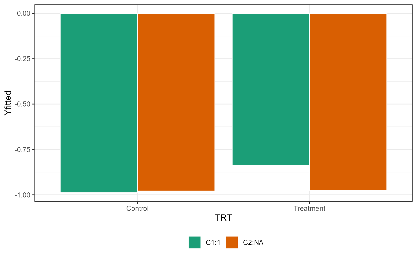
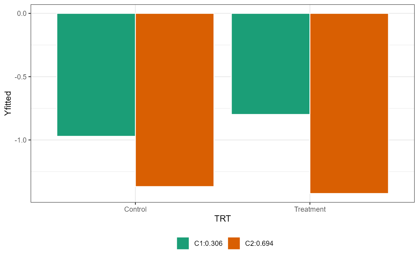
summary(res,type = "classprop")
#> classp
#>  C1  C2 
#> 306 694

flps_plot(res,type = "profile")

summary(res,type = "causal")
#>                mean     se_mean         sd         2.5%         25%         50%
#> tau0[1] -0.97110443 0.003699360 0.10703598 -1.175523442 -1.04235386 -0.97460941
#> tau0[2] -1.36827333 0.003633687 0.10962353 -1.580736339 -1.44140305 -1.36955692
#> tau1[1]  0.17263774 0.002310274 0.09473743 -0.006340285  0.10745083  0.17213108
#> tau1[2] -0.05489383 0.001289748 0.05572697 -0.168410929 -0.09096321 -0.05273357
#>                 75%       97.5%     n_eff      Rhat
#> tau0[1] -0.90334095 -0.75559665  837.1561 1.0002053
#> tau0[2] -1.29875761 -1.14158502  910.1490 0.9999325
#> tau1[1]  0.23358084  0.36991112 1681.5743 0.9997092
#> tau1[2] -0.01850267  0.05152358 1866.9011 0.9996086

flps_plot(res,type = "causal")

Latent-profile-analysis-based FLPS

Example data

data(continuous)

Fit LPA model

continuous <- continuous[c(sample(which(continuous$trt == 1), 500),
                           sample(which(continuous$trt == 0), 500)),]

res <- runFLPS(
  inp_data = continuous,
  outcome = "Y",
  trt = "trt",
  covariate = c("sex","race","pretest","stdscore"),
  lv_type = "lpa",
  lv_model = "F =~ q1 + q2 + q3 + q4 + q5 + q6 + q7 + q8 + q9 + q10",
  nclass = 2,
  stan_options = list(iter = 5000, cores = 1, chains = 2)
)

Results

summary(res,type = "classprop")
#> classp
#>   C2 
#> 1000

flps_plot(res,type = "profile")

summary(res,type = "causal")
#>                 mean    se_mean         sd       2.5%         25%           50%
#> tau0[1] -0.988596124 0.24559423 0.54101321 -1.5892444 -1.43209271 -1.3158235364
#> tau0[2] -0.979198979 0.06388208 0.15470235 -1.2587917 -1.11888637 -0.9405048631
#> tau1[1]  0.151535641 0.10277767 0.26756538 -0.3970008 -0.05717985  0.2363699003
#> tau1[2]  0.002453752 0.01615429 0.05496201 -0.1002659 -0.03606451  0.0004410687
#>                 75%       97.5%     n_eff      Rhat
#> tau0[1] -0.37972470 -0.09101688  4.852655 0.9999959
#> tau0[2] -0.85451272 -0.73751029  5.864564 1.0000767
#> tau1[1]  0.35573060  0.52997234  6.777387 0.9997000
#> tau1[2]  0.04161402  0.10911867 11.575762 0.9997540

flps_plot(res,type = "causal")