knitr::include_graphics(file.path(contents_epath, "fig1.png"))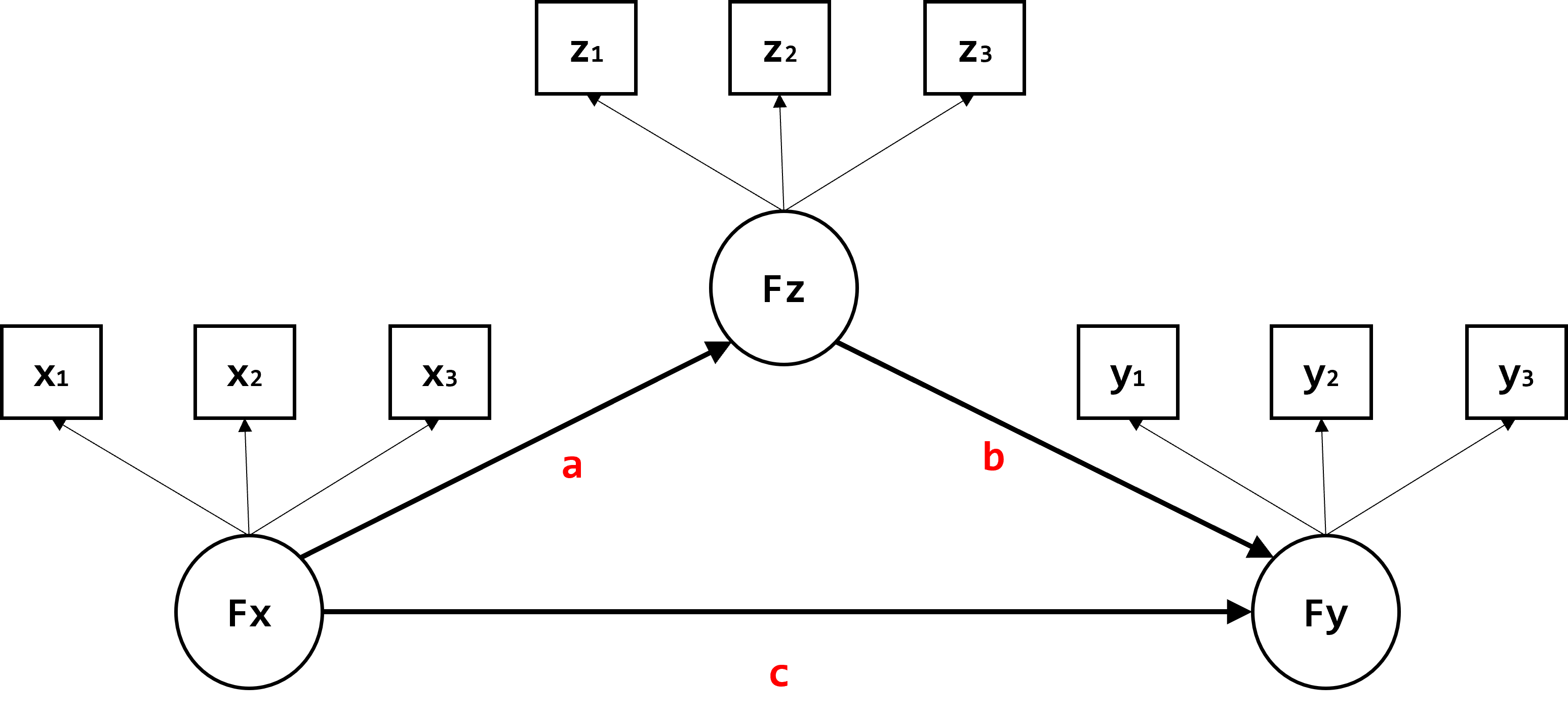
lavaanA friend of mine recently asked for help in computing power for his proposed model, as it is a necessary component of grant proposal. Power and minimal sample size are important considerations when applying for grants. The model in question was a parallel growth curve model with some mediation effects. Although I don’t have extensive knowledge about power analysis (I took a class, but…), I am aware that computing power for complex models like this requires simulation-based power analysis.
After conducting a brief search, I discovered numerous resources related to this area that I believe are worth exploring. In this post, however, I want to focus on how to perform power analysis for SEM models using lavaan, inspired by my friend’s request.
This is for my record, but I think this might be helpful to someone else as well.
For your information, there are lists of resources I think are useful as follows:
Suppose you are conducting a power analysis for a mediation model with three latent factors, and you want to determine the power of the mediation effects. To perform this power analysis using the lavaan package in R, you can follow these steps:
Set up the mediation model of interest. In this example, we have three latent factors: Fx, Fz, and Fy, with three continuous indicators per factor. The model includes a direct effect from Fx to Fy (c) and an indirect effect from Fx to Fy through the mediator Fz (a*b).
knitr::include_graphics(file.path(contents_epath, "fig1.png"))
I think the most tricky part (at least for me; and not explained much in other resources) is to determine the parameter values of each part of the model. One suggestion from Muthen and Muthen is that it should be based on previous research or preliminary results (if available). However, you may prefer to accurately specify each value and have full control over them.
Here, I briefly elaborate on how to set up and compute those values (This can be an extensive topic, and I may make another post for this when I talk about how to generate data for simulation purpose).
This involves specifying the relationships between latent factors and their indicators, represented by factor reliability. Factor reliability indicates the proportion of indicator variance explained by the latent factors (Higher means the factor better reflects the measures).
You can set different scenarios, such as low and high reliability conditions, by manipulating the factor loadings (note that because we assume standardized variables, the variance of all indicators are fixed to 1, which are easy to interpret). The variance of an indicator, \(y\), is specified by \(\lambda^2\) and \(\varepsilon\). With the variance of \(y\) standardized to 1.0, the size of \(\lambda\) determines the size of the residual variance. Squared \(\lambda^2\) reflects the proportion of variance explained by the latent factor.
\[ \sigma^2_y = \lambda^2 + \varepsilon \]
For example, if you set the reliability at 0.5 (50% of indicator variance is explained by the latent factor), the factor loading \(\lambda\) is approximately 0.7, and the residual variance is 0.5. It can simply be computed as follows:
relsize = 0.5
LAMBDA = sqrt(relsize)

expvar = LAMBDA^2
unexpvar = 1 - expvar

THETA = unexpvar
THETA
[1] 0.5LAMBDA and THETA will be used for the factor loadings and residual variances across all indicators.
Now, let’s specify the structural part of the model, which includes the paths among the latent factors (Fy, Fz, Fx).
To obtain standardized path coefficients, ensure that the latent factor variances are set to one. Standardized effects are useful for interpreting effect sizes and making comparisons. The mediation model can be expressed using the following equations:
\[Fy = c \times fx + b \times Fz + e_{Fy}\]
\[Fz = a \times Fx + e_{Fz}\]
These equations can be represented in a matrix format:
\[\begin{bmatrix} Fy \\ Fz \\ Fx \\ \end{bmatrix}=\begin{bmatrix} 0 & b & c\\ 0 & 0 & a\\ 0 & 0 & 0\\ \end{bmatrix}\begin{bmatrix} Fy \\ Fz \\ Fx \\ \end{bmatrix} + \begin{bmatrix} e_{Fy} \\ e_{Fz} \\ Fx \\ \end{bmatrix}\]
To calculate the covariance matrix, use the following equation:
\[\Sigma=(I-B)^{-1}\Psi((I-B)^{-1})'\]
where \(B\) is the matrix of structural coefficients, \[B=\begin{bmatrix} 0 & b & c\\ 0 & 0 & a\\ 0 & 0 & 0\\ \end{bmatrix}\]
, and \(\Psi\) is the residual covariance matrix, \[\Psi=\begin{bmatrix} \sigma^2_{e_{Fy}} & 0 & 0\\ 0 & \sigma^2_{e_{Fz}} & 0\\ 0 & 0 & \sigma^2_{Fx}\\ \end{bmatrix}\].
When you expand this equation, each element looks like
\[ \begin{pmatrix} c^2 \sigma^2_{Fx} + b^2 \sigma^2_{Fz} + 2acb \times \sigma^2_{Fx} + \sigma^2_{e_{Fy}} & . & . \\ b \sigma^2_{Fz} + ac \sigma^2_{Fx} & a^2 \sigma^2_{Fx} + \sigma^2_{e_{Fz}} & . \\ c \sigma^2_{Fx} + ab \sigma^2_{Fx} & a\sigma^2_{Fx} & \sigma^2_{Fx} \end{pmatrix} \]
where \(\sigma^2_{Fx}\), \(c^2 \sigma^2_{Fx} + \sigma^2_{e_{Fz}}\) (same as \(\sigma^2_{Fz}\)), and \(c^2 \sigma^2_{Fx} + b^2 \sigma^2_{Fz} + 2acb \times \sigma^2_{Fx} + \sigma^2_{e_{Fy}}\) (same as \(\sigma^2_{Fy}\)) are 1 (because we assume it’s standardized).
To obtain standardized effects, it needs to iteratively calculate the residual variances of the dependent variables (Fy and Fz).
Start by setting the residual variances to 0 in the \(\Psi\) matrix and then compute the explained variances of Fy and Fz. Subtract these explained variances from 1 to obtain the residual variances as below.
I = diag(3)
B = matrix(c(
  0, 0.4, -0.4,
  0, 0, 0.4,
  0, 0, 0
), ncol = 3, byrow = T)

PSI = matrix(c(
  0, 0, 0,
  0, 0, 0,
  0, 0, 1
), ncol = 3, byrow = T)


I.B <- I-B
IB.inv <- solve(I.B)
COV = (IB.inv) %*% PSI %*% t(IB.inv)
COV
[,1] [,2] [,3]
[1,] 0.0576 -0.096 -0.24
[2,] -0.0960 0.160 0.40
[3,] -0.2400 0.400 1.000.0576 and 0.160 reflect the explained variance of Fy and Fz, because we set PSI to 0 (residuals).
And then, calculate \(\sigma^2_{e_{Fz}}\).
diag(PSI)[2] = 1 - diag(COV)[2]
COV = (IB.inv) %*% PSI %*% t(IB.inv)
COV
[,1] [,2] [,3]
[1,] 0.192 0.24 -0.24
[2,] 0.240 1.00 0.40
[3,] -0.240 0.40 1.00Since we assume the total variance is one for all factors, to compute the residual variance, you can subtract the above explained variance from 1.
Lastly, calculate \(\sigma^2_{e_{Fy}}\). The same approach is applied.
diag(PSI)[1] = 1 - diag(COV)[1]
COV = (IB.inv) %*% PSI %*% t(IB.inv)
COV
[,1] [,2] [,3]
[1,] 1.00 0.24 -0.24
[2,] 0.24 1.00 0.40
[3,] -0.24 0.40 1.00Now, we can a full correlation matrix for our structural model relations.
$PSI
      [,1] [,2] [,3]
[1,] 0.808 0.00    0
[2,] 0.000 0.84    0
[3,] 0.000 0.00    1

$B
     [,1] [,2] [,3]
[1,]    0  0.4 -0.4
[2,]    0  0.0  0.4
[3,]    0  0.0  0.0
Use the computed \(\Psi\) matrix for the variances and residual variances of the latent factors and the \(B\) matrix for the structural parameters. The mediation effect is calculated as \(a \times b\). You can choose different values for the structural coefficients and recompute the elements of \(\Psi\) to accurately calculate the effects for power analysis.
If you want to manipulate the size of explained variance of dependent variable, you can change B and re-calculate the elements of PSI.
Once you have set up the parameter values, generating data becomes much simpler if you are familiar with the lavaan package in R. It’s worth noting that you can generate the model directly from a multivariate normal distribution using the MASS::mvrnorm function, but for consistency, we will use lavaan in this example.
pmodel <- '
Fy =~ 0.7*y1 + 0.7*y2 + 0.7*y3
Fz =~ 0.7*z1 + 0.7*z2 + 0.7*z3
Fx =~ 0.7*x1 + 0.7*x2 + 0.7*x3

Fy ~ -0.4*Fx + 0.4*Fz
Fz ~ 0.4*Fx

Fy ~~ 0.808*Fy
Fz ~~ 0.84*Fz
Fx ~~ 1*Fx

y1 ~~ 0.51*y1
y2 ~~ 0.51*y2
y3 ~~ 0.51*y3

z1 ~~ 0.51*z1
z2 ~~ 0.51*z2
z3 ~~ 0.51*z3

x1 ~~ 0.51*x1
x2 ~~ 0.51*x2
x3 ~~ 0.51*x3
'

library(lavaan)
data <- simulateData(model = pmodel,
                     model.type = 'sem',
                     meanstructure = FALSE,
                     sample.nobs = 10000,
empirical = TRUE)head(data)simulateData() function is used to generate data based on a specified model.sample.nobs = 10000).empirical = TRUE, you can obtain the exact parameter values you specified. However, when conducting simulation-based power analysis, it is recommended to set empirical = FALSE.rmodel <- '
Fy =~ 1*y1 + y2 + y3
Fz =~ 1*z1 + z2 + z3
Fx =~ 1*x1 + x2 + x3
Fy ~ c*Fx + b*Fz
Fz ~ a*Fx
# indirect effect (a*b)
indirect := a*b
total := a*b + c
'
fit <- sem(rmodel, data)To ensure that the generated data aligns with the specified model, you can use the same model syntax with the sem() function in lavaan. By examining the summary of the results, you can verify if the estimated parameters match the values you provided.
You can see exactly exactly the same values are estimated as your population data.
summary(fit, standardized = T, rsquare = TRUE)lavaan 0.6.17 ended normally after 25 iterations
Estimator ML
Optimization method NLMINB
Number of model parameters 21
Number of observations 10000
Model Test User Model:
Test statistic 0.000
Degrees of freedom 24
P-value (Chi-square) 1.000
Parameter Estimates:
Standard errors Standard
Information Expected
Information saturated (h1) model Structured
Latent Variables:
Estimate Std.Err z-value P(>|z|) Std.lv Std.all
Fy =~
y1 1.000 0.700 0.700
y2 1.000 0.020 50.155 0.000 0.700 0.700
y3 1.000 0.020 50.155 0.000 0.700 0.700
Fz =~
z1 1.000 0.700 0.700
z2 1.000 0.020 51.190 0.000 0.700 0.700
z3 1.000 0.020 51.190 0.000 0.700 0.700
Fx =~
x1 1.000 0.700 0.700
x2 1.000 0.020 51.190 0.000 0.700 0.700
x3 1.000 0.020 51.190 0.000 0.700 0.700
Regressions:
Estimate Std.Err z-value P(>|z|) Std.lv Std.all
Fy ~
Fx (c) -0.400 0.017 -24.210 0.000 -0.400 -0.400
Fz (b) 0.400 0.017 24.210 0.000 0.400 0.400
Fz ~
Fx (a) 0.400 0.015 27.478 0.000 0.400 0.400
Variances:
Estimate Std.Err z-value P(>|z|) Std.lv Std.all
.y1 0.510 0.011 46.304 0.000 0.510 0.510
.y2 0.510 0.011 46.304 0.000 0.510 0.510
.y3 0.510 0.011 46.304 0.000 0.510 0.510
.z1 0.510 0.011 47.307 0.000 0.510 0.510
.z2 0.510 0.011 47.307 0.000 0.510 0.510
.z3 0.510 0.011 47.307 0.000 0.510 0.510
.x1 0.510 0.011 47.307 0.000 0.510 0.510
.x2 0.510 0.011 47.307 0.000 0.510 0.510
.x3 0.510 0.011 47.307 0.000 0.510 0.510
.Fy 0.396 0.013 31.003 0.000 0.808 0.808
.Fz 0.412 0.013 32.210 0.000 0.840 0.840
Fx 0.490 0.015 33.639 0.000 1.000 1.000
R-Square:
Estimate
y1 0.490
y2 0.490
y3 0.490
z1 0.490
z2 0.490
z3 0.490
x1 0.490
x2 0.490
x3 0.490
Fy 0.192
Fz 0.160
Defined Parameters:
Estimate Std.Err z-value P(>|z|) Std.lv Std.all
indirect 0.160 0.009 18.006 0.000 0.160 0.160
total -0.240 0.014 -17.289 0.000 -0.240 -0.240We are all set. What we need to do is varying the sample sizes, say, from 100 up to 200 by 10 with 500 replications (more replications are needed like more than 1000). Also, you may want to use a wider range of sample sizes, a varying number of indicators, and different effect sizes or reliability levels to get a more comprehensive understanding of the power.
The target effect size is 0.4 (-0.4 for c) for each path and 0.16 for indirect effect and -0.24 (-0.4 + 0.16) for the total effect.
In practice, you may use wider range of sample sizes, varying number of indicators, and varying effect sizes or reliability.
To evaluate the indirect effects, you may have to use bootstrapping or Mackinnon’s approach, but for simplicity, I used the default pvalue of lavaan, which may be consistent with Sobel test.
sample_sizes = seq(100, 200, by = 10)
nreplication = 500
paramest <- vector('list', length(sample_sizes))
for(j in 1:length(sample_sizes)) { # j = 1
print(j)
paramest00 <- vector('list', nreplication)
for(z in 1:nreplication) { # z = 1
pmodel <- '
Fy =~ 0.7*y1 + 0.7*y2 + 0.7*y3
Fz =~ 0.7*z1 + 0.7*z2 + 0.7*z3
Fx =~ 0.7*x1 + 0.7*x2 + 0.7*x3
Fy ~ -0.4*Fx + 0.4*Fz
Fz ~ 0.4*Fx
Fy ~~ 0.808*Fy
Fz ~~ 0.84*Fz
Fx ~~ 1*Fx
y1 ~~ 0.51*y1
y2 ~~ 0.51*y2
y3 ~~ 0.51*y3
z1 ~~ 0.51*z1
z2 ~~ 0.51*z2
z3 ~~ 0.51*z3
x1 ~~ 0.51*x1
x2 ~~ 0.51*x2
x3 ~~ 0.51*x3
'
data <- simulateData(model = pmodel,
model.type = 'sem',
meanstructure = FALSE,
sample.nobs = sample_sizes[j],
empirical = F)
rmodel <- '
Fy =~ 1*y1 + y2 + y3
Fz =~ 1*z1 + z2 + z3
Fx =~ 1*x1 + x2 + x3

Fy ~ c*Fx + b*Fz
Fz ~ a*Fx

# indirect effect (a*b)
indirect := a*b
total := a*b + c
'

fit <- sem(rmodel, data)
summary(fit, standardized = T, rsquare = TRUE)
paramest00[[z]] <- parameterestimates(fit,standardized = T) %>%
filter(
(str_detect(lhs, "Fy|Fz|Fx") & str_detect(op, "^~$")) |
str_detect(op, ":=")
)
}
temp <- bind_rows(paramest00)
temp$samplesizes <- sample_sizes[j]
paramest[[j]] <- temp
}
res <- bind_rows(paramest)I made line plots for the power of each path across sample sizes.
It seems like 180 samples are needed to detect indirect effects (with the power of 80% )
sum_res <- res %>%
  mutate(
    path = paste0(lhs,op,rhs),
    detected = if_else(pvalue < 0.05, 1, 0)
  ) %>%
  group_by(path, label, samplesizes) %>%
  summarise(
    stdsize = mean(std.all),
    power = mean(detected)
  ) %>%
  ungroup()

draw_power <- function(pathname= "indirect") {
  sum_res %>%
    filter(str_detect(label, paste0("^",pathname,"$"))) %>%
    ggplot(aes(x = samplesizes, y = power)) +
    geom_point(size = 3) +
    geom_line(aes(group = 1)) +
    annotate("rect",
             xmin = -Inf, xmax = Inf,
             ymin = 0.8, ymax = 1,
             alpha = .1) +
    labs(y = "Power", x = "Sample Sizes",
         title = pathname) +
    scale_shape_manual(values = c(1:10)) +
    scale_x_continuous(breaks = seq(50, 500, by = 10)) +
    scale_y_continuous(breaks = seq(0, 1, by = 0.1)) +
    ggpubr::theme_pubclean(base_size = 14)
}ggpubr::ggarrange(
draw_power("indirect") + labs(title = "Mediation effect from Fx to Fy through Fz"),
draw_power("a") + labs(title = "b: Fz ~ Fx"),
draw_power("b") + labs(title = "b: Fy ~ Fz"),
draw_power("c") + labs(title = "c: Fy ~ Fx")
)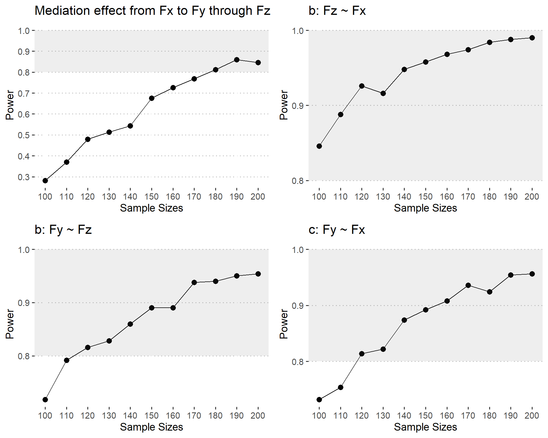
Based on the simulation results and the power curve shown in the figure, we can conclude that a sample size of at least 180 is required to detect a standardized mediation effect of 0.16 with 80% power, assuming three indicators per factor and a reliability of 0.5.
This means that if you plan to conduct a study with similar parameters (i.e., three indicators per factor, reliability of 0.5, and a standardized mediation effect of 0.16), you should aim for a sample size of 180 or higher to have a sufficient chance (80% power) of detecting the mediation effect.
It’s important to note that the required sample size may vary depending on the specific characteristics of your study, such as the number of indicators per factor, the reliability of the measures, and the expected effect sizes. Therefore, it’s always a good practice to conduct a power analysis tailored to your specific research design and parameters to determine the appropriate sample size.
By carefully considering these factors and conducting a power analysis, you can make informed decisions about the sample size needed for your study, ensuring that you have sufficient statistical power to detect the mediation effect of interest.
While there may be more advanced and sophisticated approaches to power analysis, the method described in this post is what I currently use and find effective.
It’s worth noting that this type of simulation can also be used to compute post-hoc power, where you conduct a simulation like this after data collection and analysis.
However, it’s crucial to distinguish between post-hoc power and true power. Post-hoc power analyses are generally less informative because (i) they are simply a function of the p-value and (ii) they assume that the observed effects are “true” effects.
When reporting power analyses, it’s important to focus on sensitivity power analyses, which estimate the minimum effects that the study is adequately powered (e.g., at 80%) to detect, given the analytical models and sample size. Sensitivity power analyses provide more meaningful information about the study’s ability to detect effects of interest.
If you have already collected your data and wish to conduct a power analysis, you can perform a partial power analysis by altering the path of main interest while keeping all other paths fixed across varying sample sizes. Although this may not be a complete power analysis, it is the best option in this situation.
In summary, power analysis is a crucial step in study design and interpretation. By using the simulation-based approach described in this post, you can estimate the required sample size to achieve desired levels of power for your specific research design and parameters. However, it’s important to distinguish between post-hoc power and true power, and to focus on sensitivity power analyses when reporting power. If you have already collected data, a partial power analysis can still provide useful insights, even if it is not a complete power analysis.